V2X-SenseComm

Overview

V2X-SenseComm generates multimodal V2I data from configurable urban scenes. Road maps are loaded from OpenStreetMap world data and reconstructed in Sionna ray tracing to produce synchronized near-field sensing and communication samples.

Each sample aligns scene metadata, vehicle states, camera, LiDAR, radar, GPS, ray-tracing V2I channels, and communication-side labels. Scenarios, sensing viewpoints, weather, carrier frequency, vehicle speed, and traffic settings can be configured for different ISAC tasks.

Beam Prediction

Blockage Prediction

Channel Estimation

V2X-SenseComm multimodal V2I data overview

01

Generation Pipeline

Load roads and buildings from OpenStreetMap data.
Configure traffic scenes, vehicle motion, and sensing viewpoints.
Generate synchronized sensing records and V2I channels in Sionna.

02

Data Contents

Camera images, LiDAR point clouds, radar data, and GPS positions.
Ray-tracing V2I channels and communication-side labels.
Scene metadata, vehicle states, sample indexes, and split files.

03

Supported Tasks

Beam prediction and beam management.
Blockage prediction and NLoS-aware communication.
Channel estimation, link adaptation, and multimodal ISAC learning.

Scenarios

Urban V2X scenarios

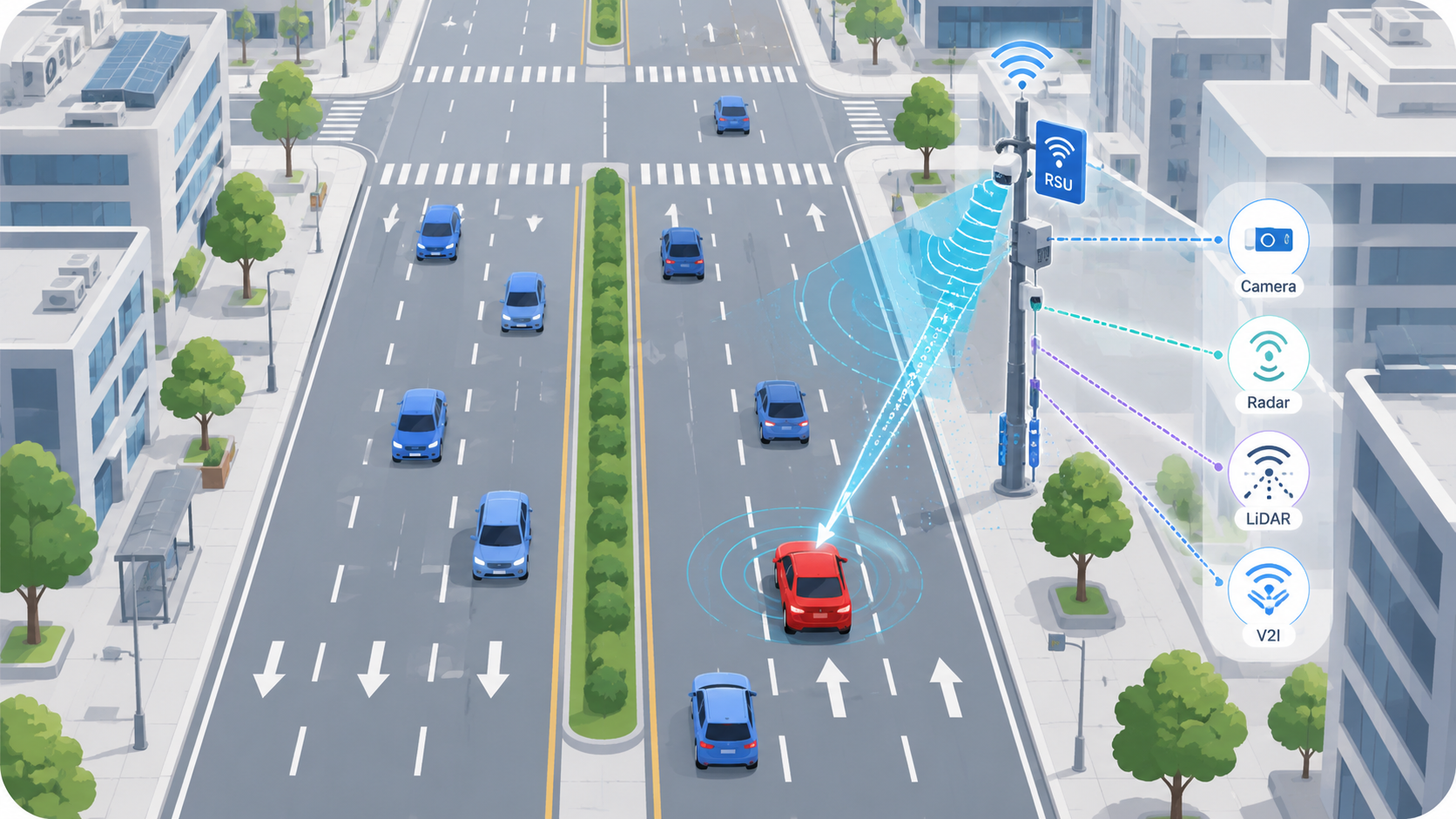
V2X-SenseComm contains 20 urban map scenes with bidirectional six-lane roads. From the inner lane to the outer lane, the baseline vehicle speeds are set to 5 m/s, 15 m/s, and 25 m/s.

20 Total Scenarios

17 Training Scenarios

3 Test Scenarios

6 Road Lanes

5-15-25-35 Lane Speeds (m/s)

3 Scenario Groups

Single-Vehicle Scene

scene_04 · Hong Kong

Dynamic Traffic Scene

scene_11 · Nanjing

NLoS Corner Scene

scene_16 · Beijing

Full Scenario Catalog

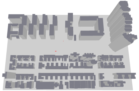
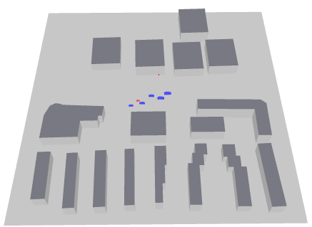
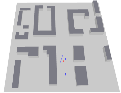
Scene ID	Region / City	Traffic Type	Propagation	Category	Dataset Split
scene_01	Beijing	Single vehicle	LoS / mixed	Single-Vehicle	Training
scene_02	Beijing	Single vehicle	LoS / mixed	Single-Vehicle	Training
scene_03	Beijing	Single vehicle	LoS / mixed	Single-Vehicle	Training
scene_04	Hong Kong	Single vehicle	LoS / mixed	Single-Vehicle	Training
scene_05	Hong Kong	Single vehicle	LoS / mixed	Single-Vehicle	Training
scene_06	Manhattan	Dynamic traffic	LoS / mixed	Dynamic Traffic	Training
scene_07	Boston	Dynamic traffic	LoS / mixed	Dynamic Traffic	Training
scene_08	London	Dynamic traffic	LoS / mixed	Dynamic Traffic	Training
scene_09	London	Dynamic traffic	LoS / mixed	Dynamic Traffic	Training
scene_10	Nanjing	Dynamic traffic	LoS / mixed	Dynamic Traffic	Training
scene_11	Nanjing	Dynamic traffic	LoS / mixed	Dynamic Traffic	Training
scene_12	Nanjing	Dynamic traffic	LoS / mixed	Dynamic Traffic	Training
scene_13	Shanghai	Single vehicle	LoS / mixed	Single-Vehicle	Test
scene_14	Shanghai	Dynamic traffic	LoS / mixed	Dynamic Traffic	Test
scene_15	Shanghai	Dynamic traffic	NLoS / mixed	NLoS Corner	Test
scene_16	Beijing	Dynamic traffic	NLoS corner	NLoS Corner	Training
scene_17	Beijing	Dynamic traffic	NLoS corner	NLoS Corner	Training
scene_18	Beijing	Dynamic traffic	NLoS corner	NLoS Corner	Training
scene_19	New York	Dynamic traffic	NLoS corner	NLoS Corner	Training
scene_20	New York	Dynamic traffic	NLoS corner	NLoS Corner	Training

Dataset

Storage format and usage

Each sample is indexed by scene, speed run, and frame. The index file links synchronized sensing files, ray-tracing communication channels, beam labels, and metadata for direct loading in Python.

visualization

A synchronized sample sequence from scene_12 / speed_+25 is visualized below. The four panels show aligned image, LiDAR, radar FFT angle spectrum, and channel-label views from the same frames.

Image

LiDAR

Radar

Channel

Directory logic

The root index files provide dataset-level access. Each scene has its own index, and each speed run stores frame-level samples. A single row points to all files belonging to the same frame, so sensing observations, channel matrices, and beam labels can be loaded together.

scene_XXUrban map scene identifier

speed_+5Vehicle speed and direction run

frame_000000Aligned sensing and communication sample

File Hierarchy

dataset/
├── index.csv
├── train_index.csv
├── test_index.csv
├── scene_01/
│   ├── index.csv
│   ├── speed_+5/
│   │   ├── meta.json
│   │   ├── index.csv
│   │   ├── camera/
│   │   │   ├── frame_000000.png
│   │   │   ├── frame_000001.png
│   │   │   ├── ...
│   │   ├── lidar/
│   │   │   ├── frame_000000.npz
│   │   │   ├── frame_000001.npz
│   │   │   ├── ...
│   │   ├── radar/
│   │   │   ├── frame_000000.npz
│   │   │   ├── frame_000001.npz
│   │   │   ├── ...
│   │   ├── gps/
│   │   │   ├── frame_000000.npz
│   │   │   ├── frame_000001.npz
│   │   │   ├── ...
│   │   ├── channel/
│   │   │   ├── frame_000000.npz
│   │   │   ├── frame_000001.npz
│   │   │   ├── ...
│   │   ├── beam_label/
│   │       ├── frame_000000.json
│   │       ├── frame_000001.json
│   │       ├── ...
│   ├── ...
│   ├── speed_-5/
│       ├── ...
├── ...
├── scene_20/

File contents description

The dataset uses run-level metadata, three-level index files, and frame-wise modality files. Each frame is stored as aligned sensing, channel, GPS, and beam-label files referenced by the index.

index.csv

dataset/index.csv: global index covering all scenes and runs.
dataset/<scene_id>/index.csv: scene-level index.
dataset/<scene_id>/<run_id>/index.csv: run-level index for one speed configuration.
Each row contains frame_idx, scene_id, run_id, weather_type, enable_occluder_cars, and paths to all frame files.

Image

camera/frame_xxxxxx.png PNG image RGB image captured from the infrastructure-side sensing viewpoint.
Image dimensions follow the camera simulator setting; each frame is aligned with LiDAR, radar, GPS, channel, and beam-label files through index.csv.

LiDAR

lidar/frame_xxxxxx.npz stores point-cloud arrays for one frame.
xyz shape: Np x 3 3D point coordinates, where Np is the number of valid points in that frame.
distance shape: Np Per-point range values aligned with the LiDAR point cloud.

Radar

radar/frame_xxxxxx.npz stores the raw radar cube for one frame.
radar_cube shape: 8 x 32 x 256 Complex radar tensor organized by chirps, antennas, and fast-time samples.

GPS

gps/frame_xxxxxx.npz stores position information for the target vehicle.
true_position shape: 3 Ground-truth vehicle position in 3D coordinates.
measured_position shape: 3 GPS-like measured position with noise.

V2I Channel

channel/frame_xxxxxx.npz stores the communication channel for one frame.
H shape: 1024 x 128 Complex V2I channel matrix generated by ray tracing. In the current configuration, the first dimension corresponds to transmit antenna elements and the second dimension corresponds to subcarriers.

Beam Label

beam_label/frame_xxxxxx.json stores codebook-search labels and beam-related annotations.
best_beam_index_3d shape: 3 Optimal beam index in the 3D codebook space, corresponding to distance, azimuth, and elevation dimensions.
best_power Scalar received power of the selected best beam.
los_exists Boolean flag indicating whether a LoS path exists.
topk_indices shape: 5 x 3 Top-5 beam candidates represented by 3D codebook indices.
topk_powers shape: 5 Beam power values associated with the top-5 candidates.

meta.json

One metadata file is stored under each speed run, such as dataset/scene_01/speed_+5/meta.json.
Key fields include scene_id, scene_source, run_id, num_frames, total_distance, and frame_interval_s.
Motion and sensor offsets are recorded by start_position, velocity_vec, sensing_tx_offset, and comm_rx_offset.
Scene conditions include weather_type, enable_occluder_cars, and num_occluder_cars.

Minimal loading example

A sample can be loaded from one row of train_index.csv or test_index.csv. The row stores relative paths to every modality, so the loader only needs to join each path with the dataset root.

Read an index file and select one sample row.
Load image, LiDAR, radar, GPS, channel, and beam-label files using the row paths.
Use the loaded arrays and JSON fields as model inputs or communication labels.

from pathlib import Path
import json
import numpy as np
import pandas as pd
from PIL import Image

root = Path("dataset")
index = pd.read_csv(root / "train_index.csv")
sample = index.iloc[0]

camera = Image.open(root / sample.camera_path)
lidar = np.load(root / sample.lidar_path)
radar = np.load(root / sample.radar_path)
gps = np.load(root / sample.gps_path)
channel = np.load(root / sample.channel_path)

with open(root / sample.beam_label_path, "r", encoding="utf-8") as f:
    beam_label = json.load(f)

points = lidar["xyz"]
radar_cube = radar["radar_cube"]
H = channel["H"]
best_beam = beam_label["best_beam_index_3d"]

Dataset

Organized for reproducible sensing-assisted communication research.

V2X-SenseComm/
├── scenarios/              # Scenario descriptions, metadata, and layouts
├── sensing/
│   ├── radar/              # Radar observations, spectra, or radar tensors
│   ├── camera/             # Reserved for future RGB images
│   └── lidar/              # Reserved for future point clouds
├── communication/
│   ├── channel/            # Ray-tracing channel responses
│   ├── beam_power/         # Beam-domain received power or beam responses
│   └── codebook/           # XL-MIMO beam codebooks
├── labels/
│   ├── best_beam_index.csv # Optimal beam labels
│   └── beam_heatmap/       # Optional beam map or heatmap labels
├── splits/                 # Train / validation / test splits
├── configs/                # Scenario, radar, channel, and codebook configs
├── scripts/                # Data generation and preprocessing scripts
└── README.md

What is included?

The dataset is designed to provide aligned sensing observations and communication labels for learning-based beam prediction.

Scenario metadata and vehicle states
Radar sensing observations or angular spectra
Ray-tracing-based communication channels
Beam-domain labels for XL-MIMO V2I links
Benchmark-ready train, validation, and test splits; validation samples are randomly split from the training scenarios

Data Format

Each sample links sensing observations, scenario metadata, and communication beam labels through a consistent sample index.

Data Loading

Example Python dataloaders will be provided for reading radar inputs, beam labels, and train/validation/test splits.

Visualization

Visualization scripts will support scenario rendering, radar spectrum visualization, and beam heatmap display.

Download Dataset

Release status and download links will be announced in the news section.

Dataset Format

Review the current directory organization and sample-level data design.

Example Samples

Browse representative scenario previews and scene categories.

Tutorials

Dataset generation tutorial

V2X-SenseComm is generated through a complete workflow from map preparation to multimodal sensing, V2I channel simulation, near-field codebook search, and beam-label generation.

Generation workflow

The pipeline starts from OSM-based map construction, adds geometry and materials in Blender, exports Mitsuba/Sionna-ready scenes, and then performs Sionna-based sensing, communication, near-field codebook search, and beam-label generation for each simulated frame.

Codebase

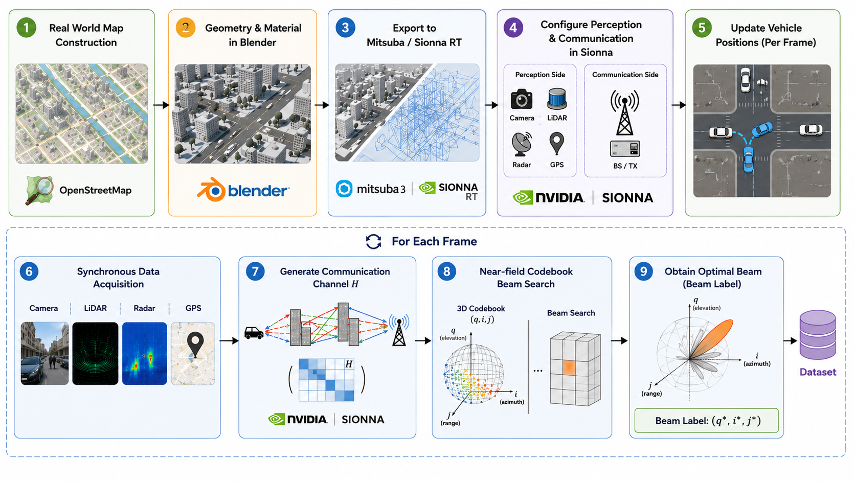
The repository separates map assets, configuration files, scene construction, sensing simulators, communication modules, and dataset writing logic. This structure makes the generation process easier to modify: scenes are selected in configuration files, sensors and channel parameters are defined once, and the pipeline executes the frame-wise data collection and labeling workflow.

Project structure

V2X/
├── run/
│   └── dataset_generation.py
├── configs/
│   ├── base_config.py
│   └── scene_map.py
├── scene_builder/
│   ├── sensing_scene_builder.py
│   ├── comm_scene_builder.py
│   ├── sensing_scene_updater.py
│   └── comm_scene_updater.py
├── sensors/
│   ├── camera_simulator.py
│   ├── lidar_simulator.py
│   ├── radar_simulator.py
│   └── gps_simulator.py
├── communication/
│   ├── channel_simulator.py
│   ├── codebook_loader.py
│   ├── beam_labeler.py
│   ├── label_writer.py
│   └── path_utils.py
├── pipeline/
│   ├── comm_pipeline.py
│   └── dataset_pipeline.py
├── maps/
├── textures/
├── codebook/
├── dataset/
└── utils/

run/

Batch-generation entry point.

dataset_generation.py traverses the configured scene list, runs each speed setting, and launches the complete data generation process.

configs/

Default settings and scene mapping files.

base_config.py defines sensing scenes, communication scenes, sensor parameters, channel settings, codebook parameters, and traffic defaults.
scene_map.py maps each scene ID to its corresponding XML map file.

scene_builder/

Scene construction and frame-wise scene updates.

sensing_scene_builder.py builds the perception scene for camera, LiDAR, radar, and GPS collection.
comm_scene_builder.py builds the communication-side scene used for V2I ray tracing.
sensing_scene_updater.py updates vehicles and mounted sensing nodes per frame.
comm_scene_updater.py updates vehicles and communication nodes in the V2I scene for each frame.

sensors/

Modality-specific simulators for synchronized sensing data collection.

camera_simulator.py renders camera images and supports weather-specific EXR environment textures.
lidar_simulator.py collects LiDAR point clouds and saves them as .npz files.
radar_simulator.py collects radar cubes and saves the raw radar_cube data.
gps_simulator.py records 3D ground-truth positions and noisy measured positions.

communication/

Communication-channel generation, codebook loading, beam search, and label writing.

channel_simulator.py calls the Sionna RT path solver to generate per-frame V2I channels.
codebook_loader.py loads the predefined near-field beamforming codebook from .npz files.
beam_labeler.py searches the codebook and outputs best beam and top-k candidates.
label_writer.py writes beam labels to frame-level JSON files.
path_utils.py provides LoS checking utilities for communication labels.

pipeline/

Pipeline modules that connect scene updates, sensing capture, channel simulation, label generation, and index writing.

comm_pipeline.py runs single-frame scene update, channel generation, beam labeling, and saving.
dataset_pipeline.py runs the full frame-wise workflow and writes samples and index files.

maps/, textures/, codebook/

Static assets used by the generation pipeline.

maps/ stores Mitsuba/Sionna-ready urban scene files.
textures/ stores EXR environment textures for weather-aware camera rendering.
codebook/ stores predefined near-field beamforming codebooks.

dataset/ and utils/

Generated outputs and shared helper functions.

dataset/ stores generated samples, metadata, labels, and train/test index files.
trajectory.py provides vehicle initial-position and velocity-vector generation utilities.
project_paths.py resolves relative paths into project-root absolute paths.

How to use

Generate SenseComm data either from the command line for scripted batch experiments or through the interactive web interface for visual configuration and sample preview.

Option 1

Command Line

Install the ray-tracing runtime, prepare the exported scene assets, select the scenes and generation parameters, then run the batch script from the project root.

# Clone the project
git clone https://github.com/fly-winder/V2X-SenseComm.git
cd V2X-SenseComm

# Install TensorFlow/Sionna RT and common Python dependencies
pip install -r requirements.txt

# Main configuration entry points
configs/scene_map.py          # SCENE_MAP: scene_id -> maps/...xml
run/dataset_generation.py     # SPEED_LIST, MOTION_AXIS, WEATHER_TYPE, OUTPUT_ROOT
configs/base_config.py        # camera/lidar/radar/gps, channel, array, codebook

# Run dataset generation
python run/dataset_generation.py

Option 2

Web Interface

Use the Streamlit interface to configure scenes, trajectories, sensor modules, communication settings, and output paths without editing configuration files manually.

# Clone the project
git clone https://github.com/fly-winder/V2X-SenseComm.git
cd V2X-SenseComm

# Install dependencies
python -m pip install -r requirements.txt

# Start the generation UI
python -m streamlit run app/generator_app.py

Open http://localhost:8501 in your browser, configure the generation settings, and click Run Generation.

V2X-SenseComm interactive web interface for dataset generation — The interface supports both Basic Mode and Advanced Mode and allows users to preview the generated multimodal sensing and communication data.

Code

Code repository

fly-winder/V2X-SenseComm

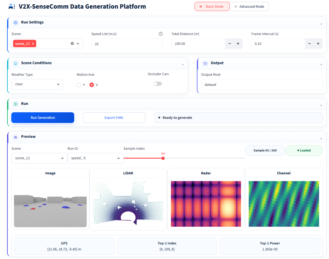
The code will be released after publication.

Publications

Publications will be updated after the related papers are available.

Download

View Dataset